Using Dynamic Pile Driving Formulas on Site
I thought I’d post this blog as it is directly relatable to my thesis topic and highlights the risk of ‘boundaries’ regarding geotechnical engineers and pile design.
The marine piling package is well underway on my project, with 5 piles installed to date. I am not overseeing this package (I am focussed on substructure works on the eastern bank of the site) but have been keeping myself up to date with the marine piling QA as my thesis is aimed around pile driving formulas and will use primary data from our pile driving records/CAPWAP analyses.
A few weeks back, one of our piles (P1-P09-PSP-01) was driven to design depth but failed to reach End of Dive (EOD) capacity, recording a set of just 5.1mm per blow at ~280kj of energy. This pile is an open-ended steel tube with a diameter of 1600mm, pile wall thickness of 25mm and pile shoe of 1m long by 50mm wall thickness. It is designed to carry a geotechnical design load of 21MN.
Piles have been driven using an IHC S280 hammer, and was initially driven with Pile Driving Analyser (PDA) equipment to a penetration of 21.77m (-32.36m RL). The PDA EOD indicated that the pile had an inadequate resistance at this depth. The PDA equipment had to be removed due to the risk of water damage (i.e. the gauges were at risk of being submerged in the River). A CAPWAP analysis was carried out on one of the final blows at this stage of re-driving, also proving inadequate capacity.
Though both a borehole was taken at each pier location and the pile itself was fabricated with an extra 2m length to mitigate risk of failing to reach capacity at design RL, this situation highlights the risk of certainty in geotechnical boundaries.
The pile was driven further without PDA monitoring and the set was monitored using survey. The pile was driven to a final toe level of -32.8m RL. The final set achieved was 1.6mm (per blow) at maximum hammer energy (~280 kJ). This was positive, suggesting the basalt rock layer had been established.
For the project to date, PDA testing and CAPWAP analysis have been undertaken on all previous marine piles to confirm capacity. This has enabled correlations to be developed to PDA/CAPWAP to pile installation parameters (i.e. you can use sets achieved on previous piles to estimate pile capacity). As no PDA equipment was attached for the final driving of the pile (and thus no possibility of CAPWAP analysis), an alternate approach to pile capacity verification was required.
Without going into too much detail, hundreds of dynamic pile driving formulas have been derived since the mid to late 1800s. In Victoria, the Hiley Formula is referenced for use in VicRoads publications, which is dated and requires input of several parameters. One such input is the Temporary Compression (TC) measurement of the pile (effectively the energy lost during hammer impact due to elastic compression in the pile, soil and cap). TC energy losses are on of two types on losses experienced, the other be Newtonian Impact Theory (effectively a coefficient of restitution that is used to indicate how much of the original kinetic energy remains after the impact of two objects)
TC could not able to be recorded onsite due to the difficulty obtaining this measurement due to the pile becoming submerged and the hammer sleeve ‘covering’ the top of pile. This prevented the Pile Driving Monitor (PDM) from being used to record TC.
Therefore, the geotechnical engineers required use of a pile driving formula that does not incorporate TC. Stringent rules allow for this and is only considered appropriate in cases where:
-
- There is a high proportion of piles subjected to PDA/CAPWAP;
- Hammer energy measurement is undertaken to confirm hammer performance;
- There is a high level of engineering supervision and the standard of piling QA is high.
These requirements were considered met so the geotechnical engineers decided that the ‘Gates Pile Driving’ Formula (developed in 1957) would be used to allow estimation of pile resistance. The Gates Formula is as follows:
𝐺𝑎𝑡𝑒𝑠 𝑅𝑒𝑠𝑖𝑠𝑡𝑎𝑛𝑐𝑒 𝐹𝑎𝑐𝑡𝑜𝑟 = 27 ∗ √𝑒ℎ ∗ 𝐸 ∗ (1 − 𝑙𝑜𝑔10 (s/25.4))
where: s is set in mm
eh is hammer efficiency (assessed as efficiency of energy transfer to the pile from PDA measurements on other representative piles)
E is the hammer energy delivered to the pile.
As the Gates Formula was developed in US units (i.e. kips, ft) the formula does not result in a resistance in metric units (i.e. kN). To avoid the need to convert all units to US and redefine the constants in the equation, the Gates Formula was used to evaluate a ‘Gates Resistance Factor’ which is proportional to the estimated resistance. Importantly, this is subsequently correlated to CAPWAP resistance.
A correlation factor is necessary between the GRF and the PDA/CAPWAP capacities determined from analysis on representative tested piles (i.e. piles already installed). This correction factor is termed Gates Correction Factor (GCF) and is calculated as:
𝐺𝐶𝐹 = CAPWAP Resistance / 𝐺𝑅𝐹
|
Test No. |
Toe Level (Test) | Pile Penetration (Test) |
Driving Stroke |
EOD
Driving Set |
Driving TC |
Test Type |
Test Set |
EMX |
RMX |
Potential Energy |
Hammer Efficiency |
| – | m RL | m | mm | mm | mm | – | mm | kN- m | kN | kN-m | – |
| C1-P03- PSP-03 EOD |
-31.53 |
19.33 |
2040 |
0.50 |
13.90 |
EOD |
0.5 |
248 |
33529 |
280.2 |
88% |
| C1-P03- PSP-04 EOD |
-32.45 |
15.65 |
1600 |
1.40 |
12.60 |
EOD |
1.4 |
218 |
28303 |
219.7 |
99% |
| C1-P03- PSP-04 RST | -32.45 | 15.65 | 1700 | 1.40 | 12.60 | RST | 0.7 | 228 | 29517 | 233.5 | 98% |
| C1-P03- PSP-04 RDV |
-32.45 |
15.65 |
2040 |
1.40 |
12.60 |
RDV |
1 |
269 |
32231 |
280.2 |
96% |
| C1-P03- PSP-02 EOD |
-35.10 |
13.00 |
1600 |
2.30 |
11.70 |
EOD |
2.3 |
207 |
19863 |
219.7 |
94% |
| C1-P03- PSP-02 RST | -35.10 | 14.50 | 2040 | 2.30 | 11.70 | RST | 1.3 | 269 | 25067 | 280.2 | 96% |
| C1-P03- PSP-01 EOD |
-35.07 |
13.20 |
1455 |
2.80 |
10.20 |
EOD |
2.8 |
191 |
18827 |
199.8 |
96% |
| C1-P03- PSP-01 RST | -35.07 | 14.30 | 2040 | 2.80 | 10.20 | RST | 1.7 | 270 | 24708 | 280.2 | 97% |
| P1-P09- PSP-01 RDV |
-32.36 |
21.77 |
2040 |
5.10 |
– |
RDV |
5.1 |
276 |
22475 |
280.2 |
98% |
The table above demonstrates the results of the testing conducted (EOD and CAPWAP) on the 4 previously installed piles for correlation for Gates. The table below shows the pile resistance factor values calculated from the Gates Formula, as well as capacity evaluated from CAPWAP and the GCF.
For all tests (excluding Pile C1-P03-PSP-03 EOD which is considered unrepresentative) the energy efficiency ranged from 94 to 99% (an important parameter for formula input), with an average of 96.8. A Lower Bound efficiency of 94% was adopted in estimating resistance for pile P1-P09-PSP-01.
|
Test No. |
Gates Resistance Factor |
CAPWAP Compressive Capacity |
GCF |
| – | – | (kN) | |
| C1-P03-PSP-03 EOD | 1149 | 33500 | 29.1 |
| C1-P03-PSP-04 EOD | 900 | 25555 | 28.4 |
| C1-P03-PSP-04 RST | 1044 | 29570 | 28.3 |
| C1-P03-PSP-04 RDV | 1065 | 32280 | 30.3 |
| C1-P03-PSP-02 EOD | 792 | 19700 | 24.8 |
| C1-P03-PSP-02 RST | 1014 | 25080 | 24.7 |
| C1-P03-PSP-01 EOD | 730 | 18790 | 25.7 |
| C1-P03-PSP-01 RST | 966 | 24670 | 25.6 |
| P1-P09-PSP-01 RDV | 761 | 22315 | 29.3 |
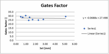
The Gates resistance values are generally seen as lower than the CAPWAP resistances with GCF values from 24.8 to 30.3. These are plotted against pile set below to provide a line of best fit of pile set against the Gate Factor. Using this and the set obtained at EOD (1.6mm) for pile P1-P09-PSP-01, the GCF equates to ~27.
Using the below parameters, The Gates Pile Driving Formula estimates a resistance of 26,173kN at end of redrive.
Set = 1.6mm
Hammer Energy = 280kJ (IHC S280) Hammer Efficiency = 94% (LB)
Gates Correlation Factor = 27
This is well above the required capacity of the pile (~21MN) and is therefore considered competent. In addition to this, the previous piles have demonstrated a ‘set up’ (refer to my previous post) of 15%-31% increase over 24 hours (minimum required time between EOD and Restrike Test (RST)) – See table below. This suggests further assurance to capacity and thus QA of the pile.
|
Test No. |
Compression Shaft Resistance |
Toe Resistance |
Compression Capacity |
Toe Level (Test) |
Shaft capacity improvement (%) |
Overall Capacity Improvement (%) |
| kN | kN | kN | mRL | |||
| C1-P03-PSP-04 EOD | 8055 | 17500 | 25555 | -32.450 |
146% |
115% |
| C1-P03-PSP-04 RST | 11770 | 17800 | 29570 | -32.450 | ||
| C1-P03-PSP-01 EOD | 7390 | 11400 | 18790 | -35.070 |
161% |
131% |
| C1-P03-PSP-01 RST | 11970 | 12700 | 24670 | -35.070 | ||
| C1-P03-PSP-02 EOD | 7700 | 12000 | 19700 | -35.100 |
150% |
127% |
| C1-P03-PSP-02 RST | 11580 | 13500 | 25080 | -35.100 | ||
| P1-P09-PSP-01 RDV | 9765 | 12550 | 22315 | -32.363 |
152% |
124% |
| Average | ||||||
The use of the Gates Formula on site to assure capacity of this pile has been, coincidently, very useful for my Thesis and demonstrates alternate methods of assuring quality. The importance appears to be in the ability to both/either accurately measure parameters/input data on site and correlate results with a data set. Without having yet asked, I wonder what the solution might have been had this been the first pile? Maybe install further piles and hope to achieve resistance and use the parameters obtained to correlate as was in this case? Or would they have bit the bullet and spliced the pile on site – rather tricky being in a marine environment from a barge, especially given the high QA regime and Workplace Health & Safety controls?

Looks like an extract from your thesis!
Without commenting too much on the specific case some generalities….
1 Can a dynamic test ever theoretically predict static performance?
2 In what circumstances would the dynamic testing be influenced by, say , dilatational effects i.e. temporary increase in penetration resistances associated with the dynamic nature of the testing?
3 Equally, in what circumstances would a dynamic elastic model come closest to a sensible model for static pile resistance…and do they exist here?
4 Why does UK practice largely require static confirmation of dynamic q.a. ?
Hi John,
It appears to have been a fantastic coincident for me (not so much the contractor). I plan to incorporate into my thesis as this is one of the formulas I am looking at.
In response to your questions:
1. If the theory is good, then yes (I suppose). However, for practical circumstances it is essentially just a correlation … so no(ish)?
2. I suppose there could be two?
The first would be in a dilative soil/sand where pore water pressures actually decrease during driving, thus increasing effective stresses. The dynamic test would therefore offer a higher resistance than the longer term. As dynamic testing is only applicable to the time of testing, over estimation of pile capacity would be the result.
The second, I think, would be more directed at cycling on the pile (tidal/waves/environmental/seasonal) – i.e. ‘load cycling’ will cause a cycle of dilation and contraction.
3. I suppose the difficulty is applying an appropriate stiffness in an elastic model. This would change along the length of the pile as the strain varies, thus changing the stiffness. So i’d conclude that it would form a sensible model where an appropriate stiffness factor could be applied along the length of the pile?
4. I guess this ties in to my response to the first. Dynamic tests are effectively just correlations rather than proof. So you’d need something (i.e. a static load test) to calibrate against. I suppose here, in Victoria, they rely on being able to correlate their dynamic testing with previous load tests assuming similar ground conditions?